Final Project Report
Group: Xiaohe Niu and Véronique Kaufmann
Content
Features Véronique Kaufmann
- Directional Light Emitter
- Images as Textures
- Normal Mapping
- Henyey Greenstein Phase Function
- Emissive Participating Media
- Homogeneous Participating Media
- Spectral Rendering
Graded Features Véronique Kaufmann
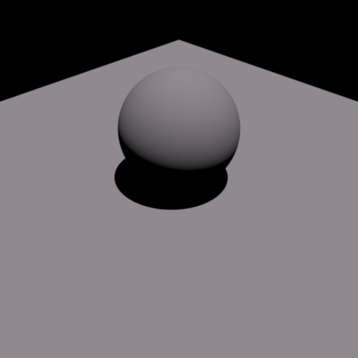
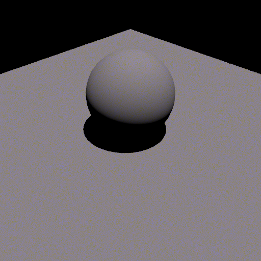
Directional Light Emitter (5)
Relevant Files
src/directionalLight.cpp, src/scene.cppImplementation
The implementation of the directional light emitter (or distant light, as it is called in some renderers) is straightforward. The evaluation always returns the power of the emitter. The only tricky part is the sampling. To be able to build a shadow ray, we need a point outside of the bounding sphere of the scene. To do this, we added a variable "m_WorldRadius" to the emitter class, and set it every time an emitter is added to the scene (this happens in scene.cpp, where we have access to the scene bounding box). The rest of the implementation closely follows that of a pointlight.
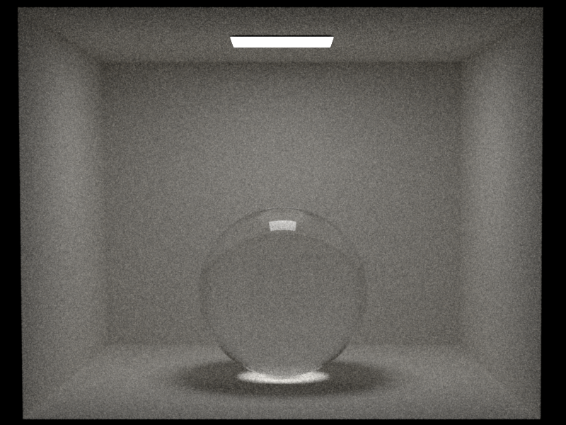
Validation
The following renderings show a comparison between my implementation and mitsuba2. Since directions are defined slightly differently in mitsuba and nori, we have to swap the first 2 coordinates of the direction-vector when using mitsuba to get the same output image. Further, we use the same radiance value for both and, as we can see, achieve the same result.
Images as Textures (5)
Relevant Files
imagetexture.cppImplementation
To use images as textures, we include lodepng, a png-loader for C++. When an image texture is instantiated, we then first load the texture given the relative path to it. Lodepng will then load the image in a char array. This will store the texture in an array of chars. To evaluate the texture, we first transform the (u,v)-coordinates to image coordinates (s,t), as we already to implement the checkerboard texture. After that, we compute the index to access in the texture array given s and t, as well as the height and width of the image texture. This gives us a 3D vector (R, G, B), that we normalize by dividing it by 255 to get it into [0, 1]. This will return the colors in sRGB format, so we have to transform it back to linear RGB. We do that by using the function provided by nori.
Validation
Below you find renderings using nori and mitsuba for the same texture. Because mitsuba and nori don't use exactly the same coordinate frames, I also have to shift the texture by 0.5 when loading it into mitsuba in order to achieve the same result.
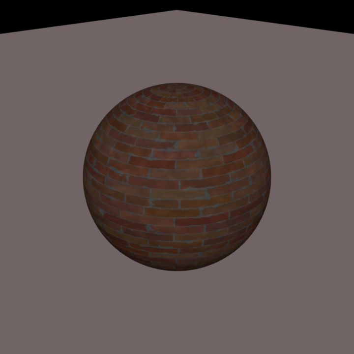
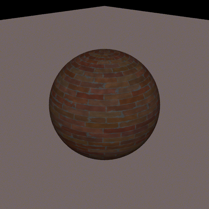
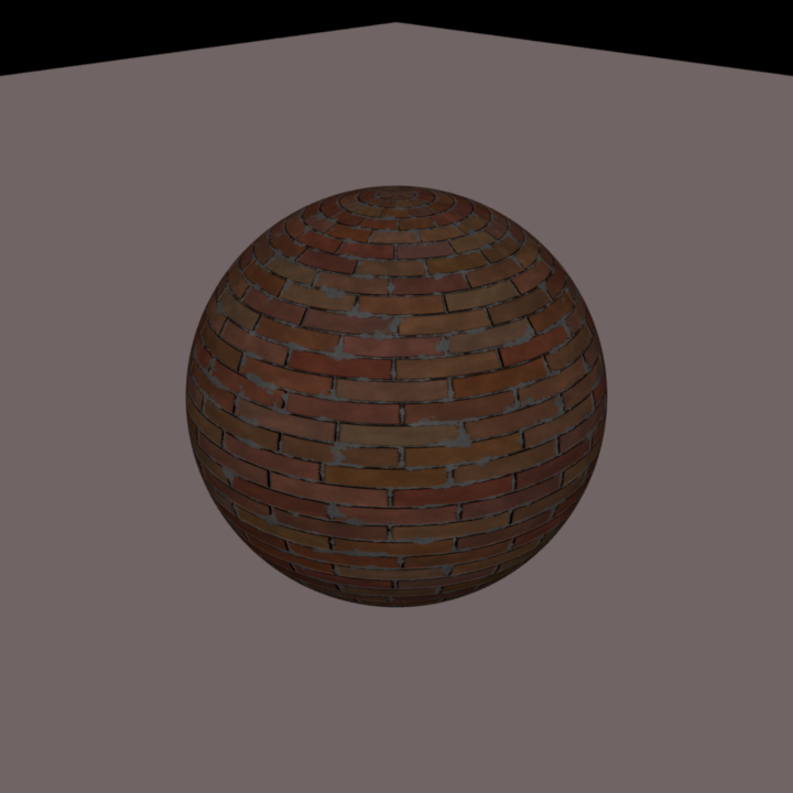
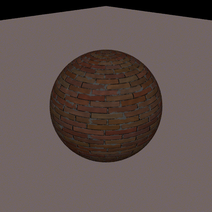
Normal Mapping (5)
Relevant Files
include/nori/shape.h, src/bvh.cpp, src/mesh.cpp, src/sphere.cppImplementation
To add normal mapping to the existing nori implementation, we add three functions to shape.h. One of them evaluates the normal map. One to load a texture and one to evaluate it. These two are basically the same as we used for the image texture feature, except that evaluation now returns a direction instead of a color. Since we already have the images as texture feature, we load the normal map as a png as well. There is currently no support for other formats of bumpmaps, but this could be extended without additional effort. The loading function is called when a mesh or a shape (in our case the sphere) is created. We add a second function that updates the shading frame. This will be called after calling "SetHitInformation". This function computes the tangent and bitangent using the normal vector extracted from evaluating the bump map, and then update the shading frame accordingly. We call this function from bvh.cpp after setHitInformation is called.
The main idea behind the implementation was to leave the individual shape classes (Mesh, Sphere, ..) as untouched as possible.
Validation
Below you can find renderings of a sphere with a brick texture applied to it. You can see a four-way comparison showing the texture only as well as the texture and with the normal map applied, rendered once in nori and once in mitsuba for validation.
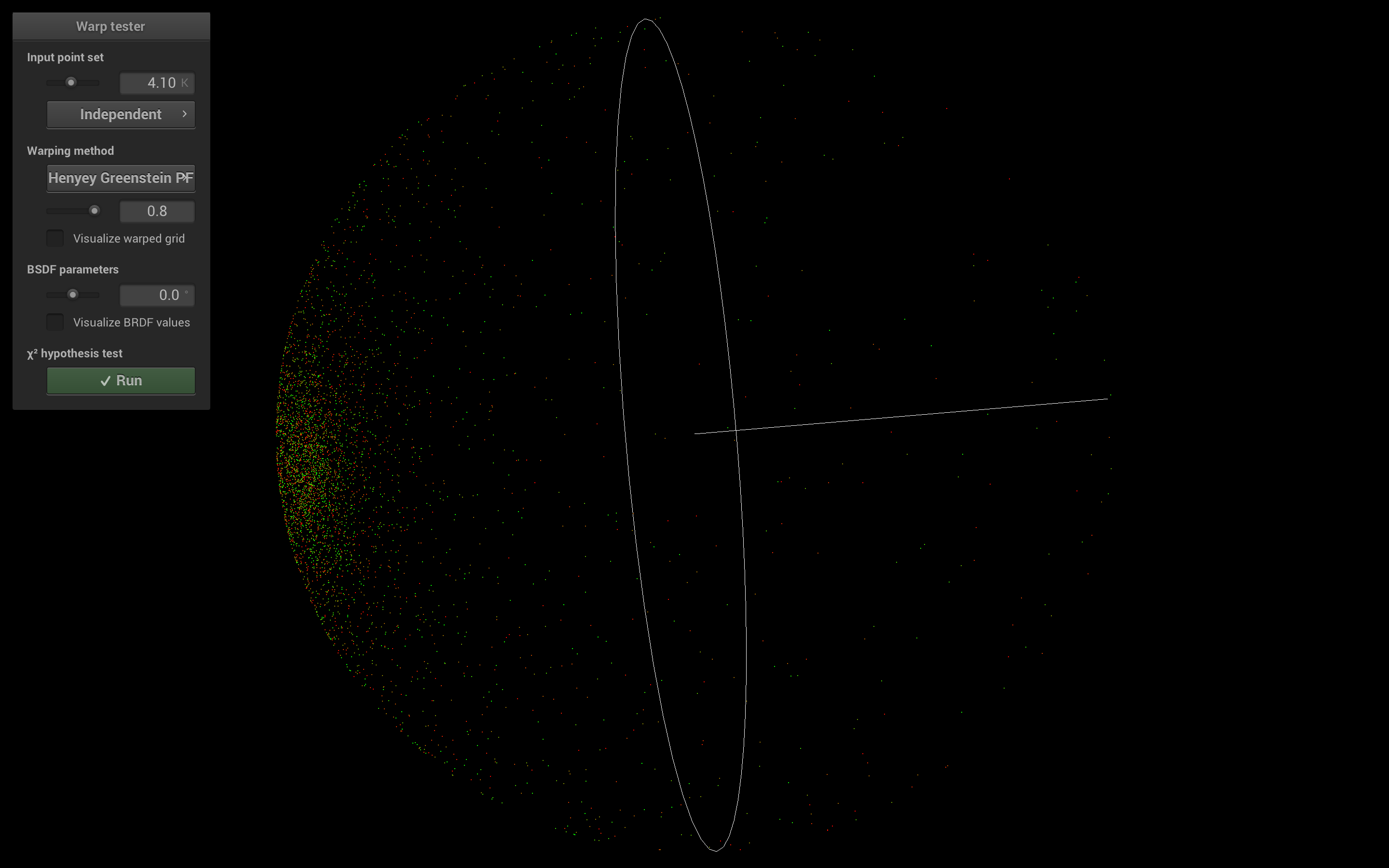
Henyey Greenstein Phase Function (5)
Relevant Files
include/nori/phase_function.h, include/nori/henyey_greensteinImplementation
We implement the Henyey Greenstein Phasefunction to use with participating media (see next homogeneous media). To do this, we first create a new header class for phase functions. This allows to extend by other phase functions if desired. The implementation closely follows pbrt and mitsuba. We have a function to sample, and one to get the pdf (PhaseFunction::p). Both of these take a PFQuery record as input, where the sample function will set the outgoing direction wi.Validation
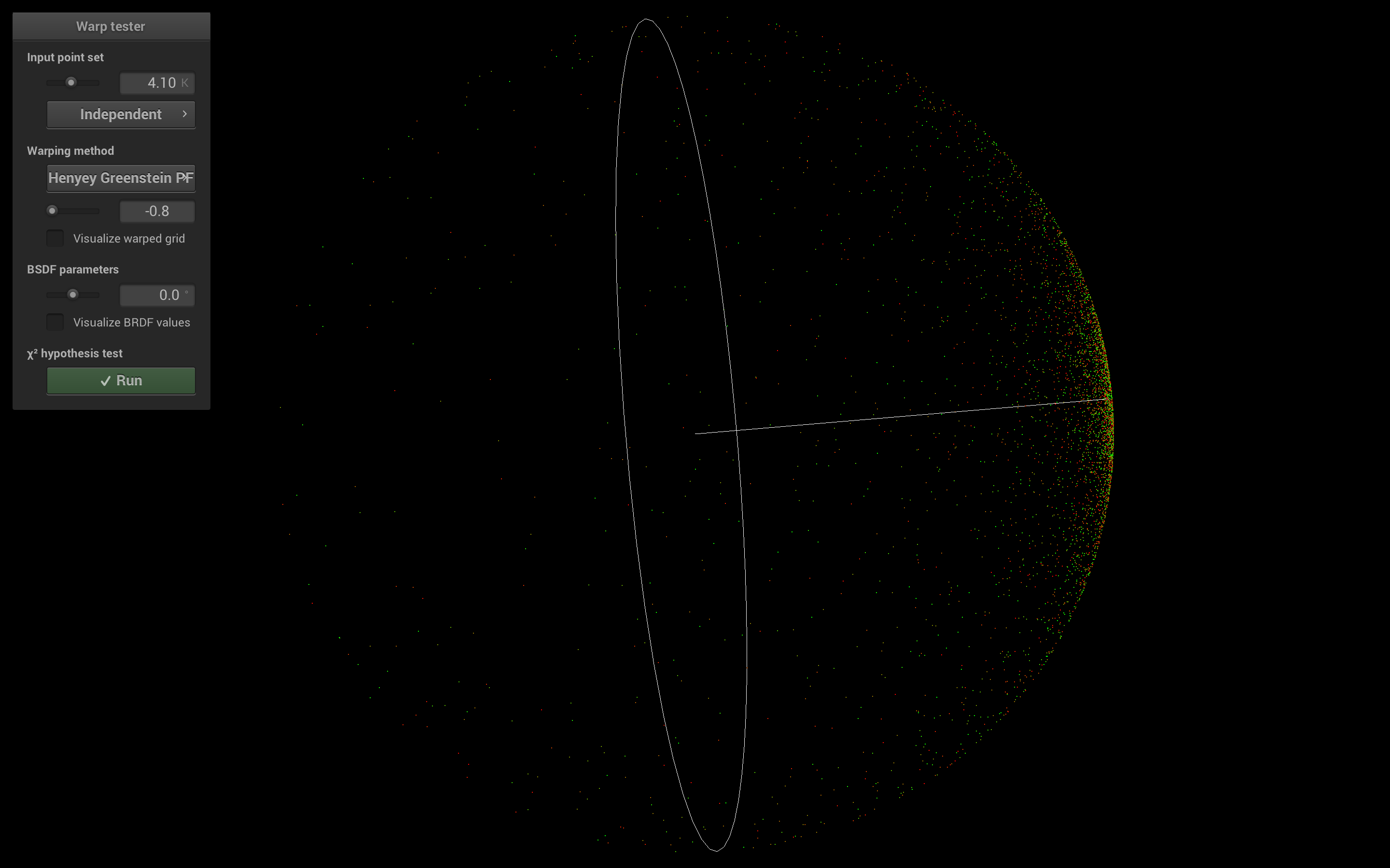
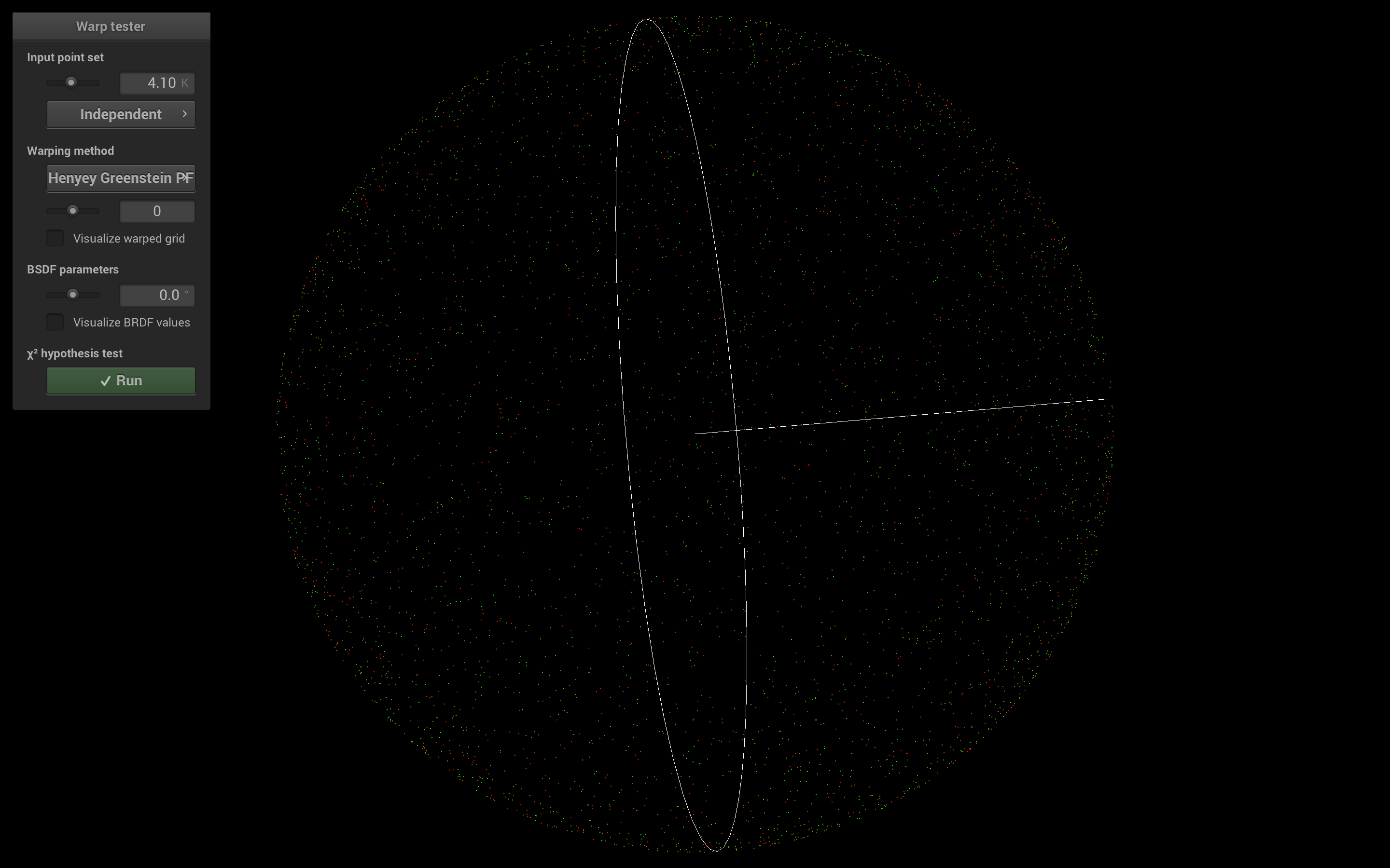
Below we first show a rendering of three spheres using the same medium-parameters, but different g for the Henyey Greenstein phase function. The g values are (from left to right): -0.8, 0.0, 0.8.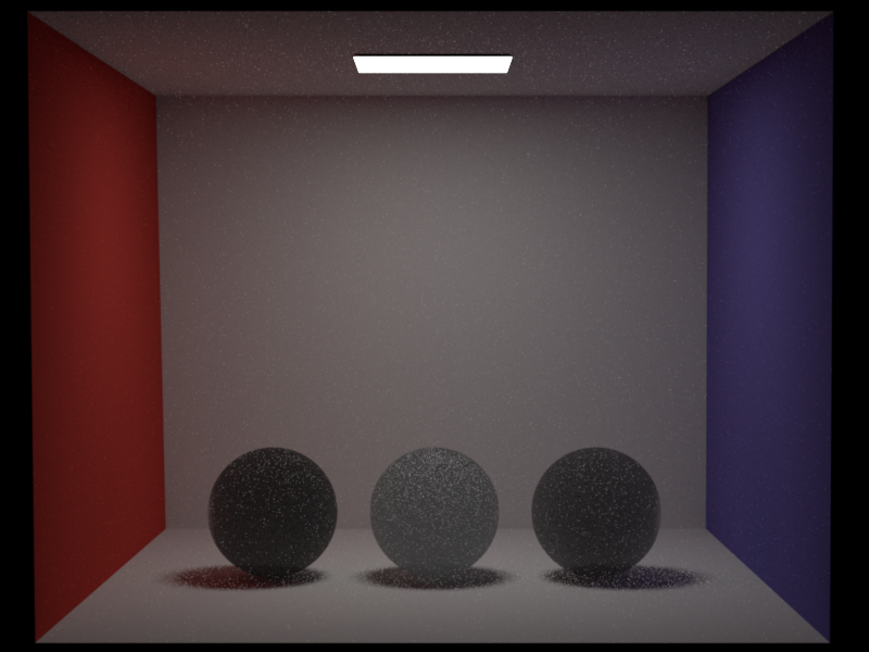
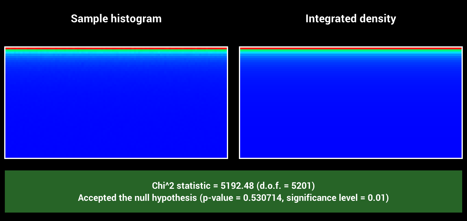
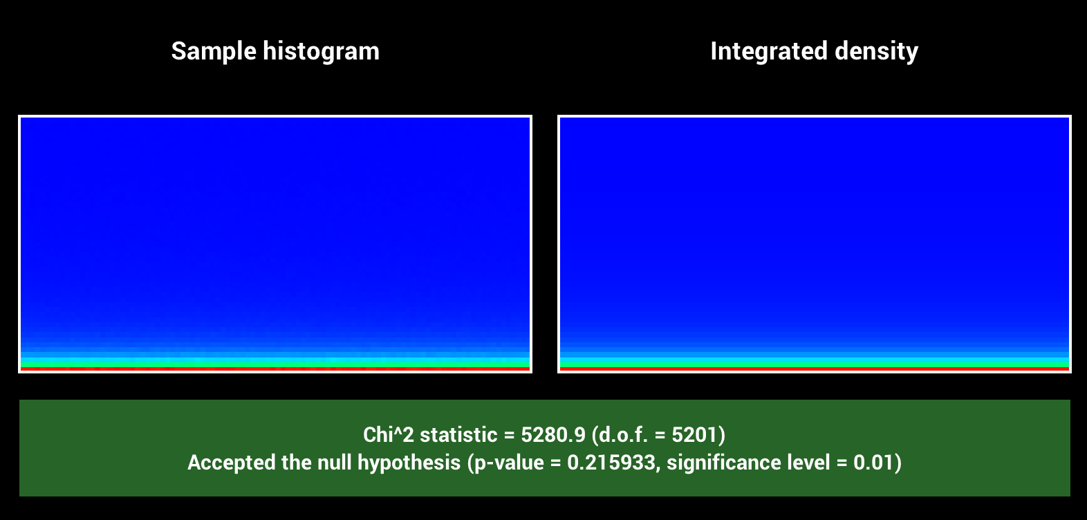
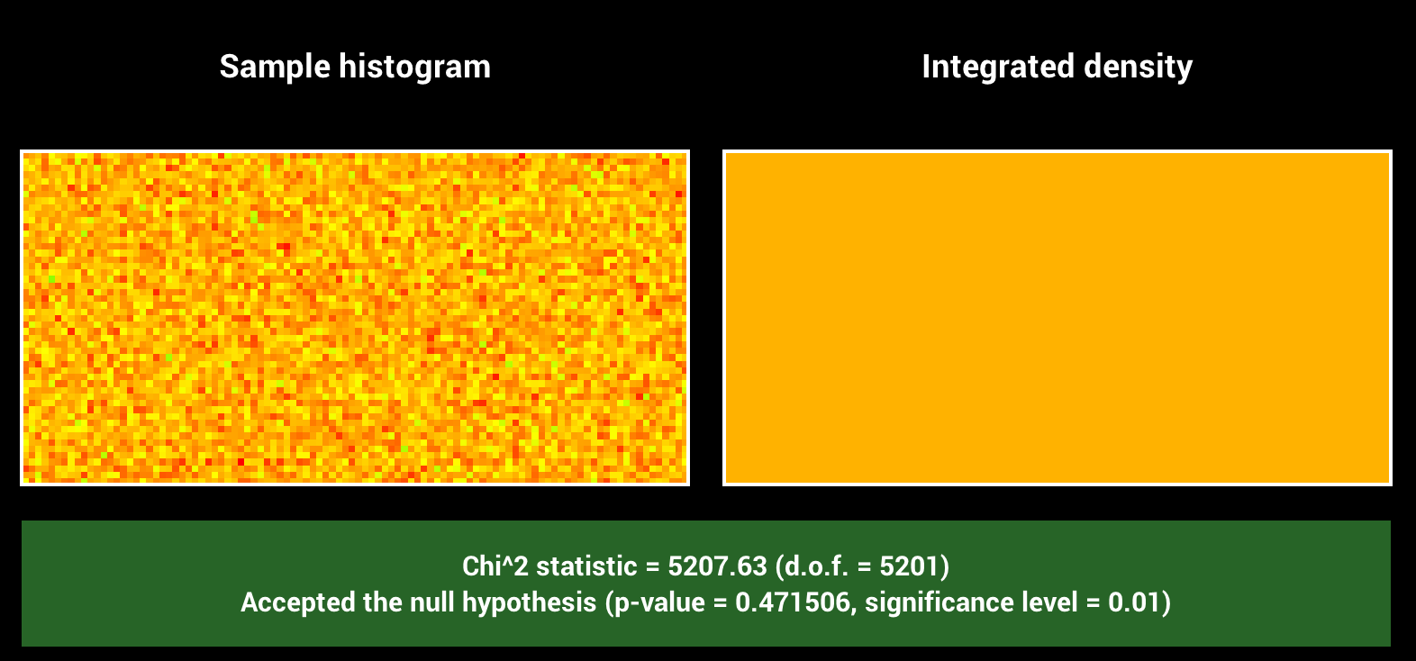
For validation, we modified warptest.cpp to show the distribution of the henyey greenstein sample methods. Below you can see examples for g equal to 0, less than 0 and larger than 0. For all possible values, we pass the chi2 tests.
Emissive Participating Media (10)
Relevant Files
src/emissive_medium.cppImplementation
To support emissive media in nori, we extend our definition of a medium such that we can attach an emitter to it. We then define a new emitter called "Emissive Medium". We then override the addChild method of our medium, to support adding an emissive medium emitter to it. The general medium type is described in the next section about homogeneous media.
The emissive medium can now be treated like an emitter in the our medium path tracer, but at the same time, it keeps its properties as a medium. To evaluate the emissive medium emitter, we simply integrate over the path between the intersection point, and the exit point of the ray going through this point into the medium. Since we only have homogeneous, the computation is straight forward.
We now also have to define sampling for homogeneous volumes. For evaluation and sampling of the emissive medium emitter, we closely follow this paper . Evaluation simply integrates over the radiance along the ray crossing through the medium. For sampling, we sample a point inside the volume of the medium (so far we do this uniformly, however with more time the properties of the medium could be included). We then compute the radiance along the ray between the reference point and the sample point, that is within the medium.
Validation
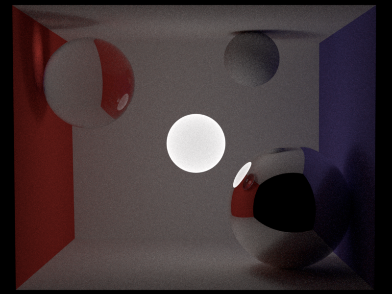
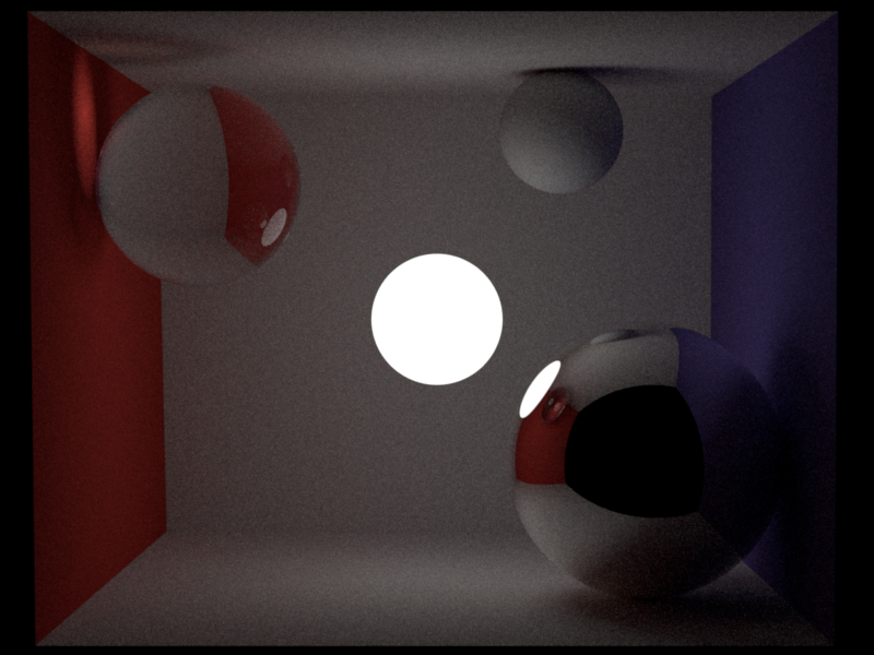
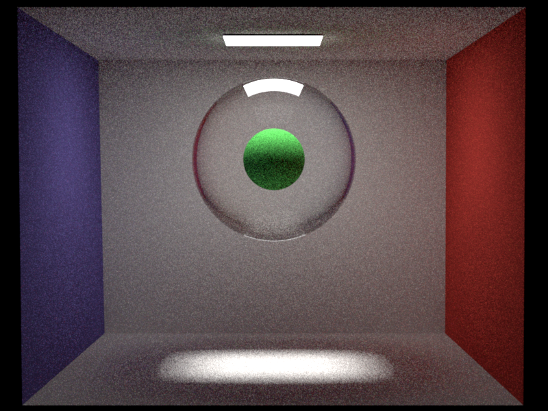
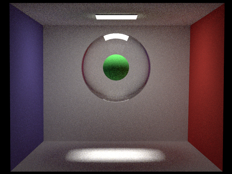
For validation I provide a scene below with some spheres with different bsdfs (mirror, diffuse, dielectric) and an emissive medium sphere in the middle. We can see from the shadow how the medium emits light in all directions. Further, we also show a comparison to the same scene rendered with an area light instead of the emissive media. We can see the similarity, however we cannot expect the two images to look identical, since the area light samples only the surface, while the medium also considers the volume.
We also show a comparison to using an area emitter in the shape of a sphere. It has to be said that the results here are not supposed to be exactly the same, since the emissive medium can also be sampled inside the medium, while the area light is only a surface.

Homogeneous Participating Media (15)
Relevant Files
include/nori/medium.h, include/nori/shape.h, src/homogeneous_participating_medium.cpp, src/medium_path_mis.cpp, src/medium_path_mats.cpp, src/shape.cppImplementation
Many scenes require the support of not only shapes and surfaces, but participating media. The support of such media requires some setup. First, we create a medium class of type EMedium. Each medium has a phase function attached. We then create a homogeneous medium that is very similar to PBRT, where we use Beer's law to compute transmittance within the medium. Further, the homogeneous medium uses the Henyey Greenstein phase function we computed earlier. The medium also has a function to sample from it.
To render the medium, we also implement a new integrator. We provide both a version using multiple importance sampling, and one that doesn't, in order to show that multiple importance sampling works and improves the result. For each ray iteration, we check if the origin of the ray is inside a medium. This means, we have some interaction even if there was no intersection. This function will also return true if we are on the boundary of a medium, which solves the problem of entering/exiting the medium. If the origin of the ray is inside a medium, we use the phase function to sample the direction of the next ray. We then compute the contribution of the medium and add it to the radiance term, weighted by the mis-weight.
If we are in a medium, we compute the direction and mis-weights based on the sampled direction and the pdf of the phase function. If we are not in a medium, we use the bsdf as we did in the assignment to implement of path_mis.cpp.
Validation
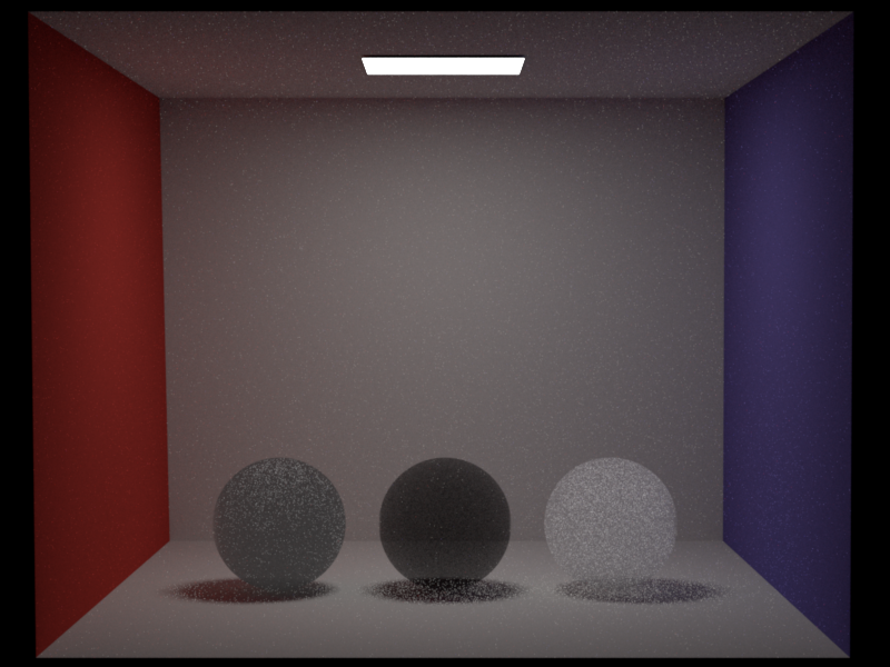
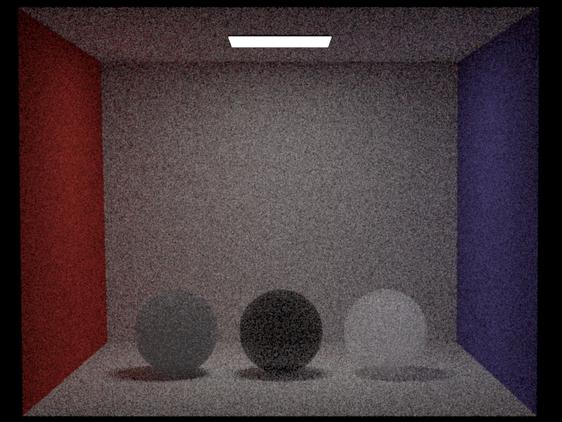
The following rendering uses an isotropic phase function to make comparison easier. We compare the nori renderings to renderings using mitsuba2, both using an independent sampler with 200 samples per pixel.
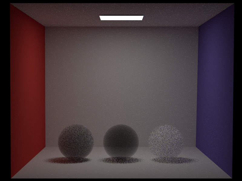
The following image shows 3 different types of media. These are (left to right): sigma_s = 5, sigma_a = 0, sigma_s=5, sigma_a = 5, sigma_s=0, sigma_a=5.
Below we also show the difference between the naive volumetric path tracer and the path tracer using multiple importance sampling between the phase function and the emitter (in case of a medium interaction), or between the bsdf and the emitter (in case of a surface interaction).
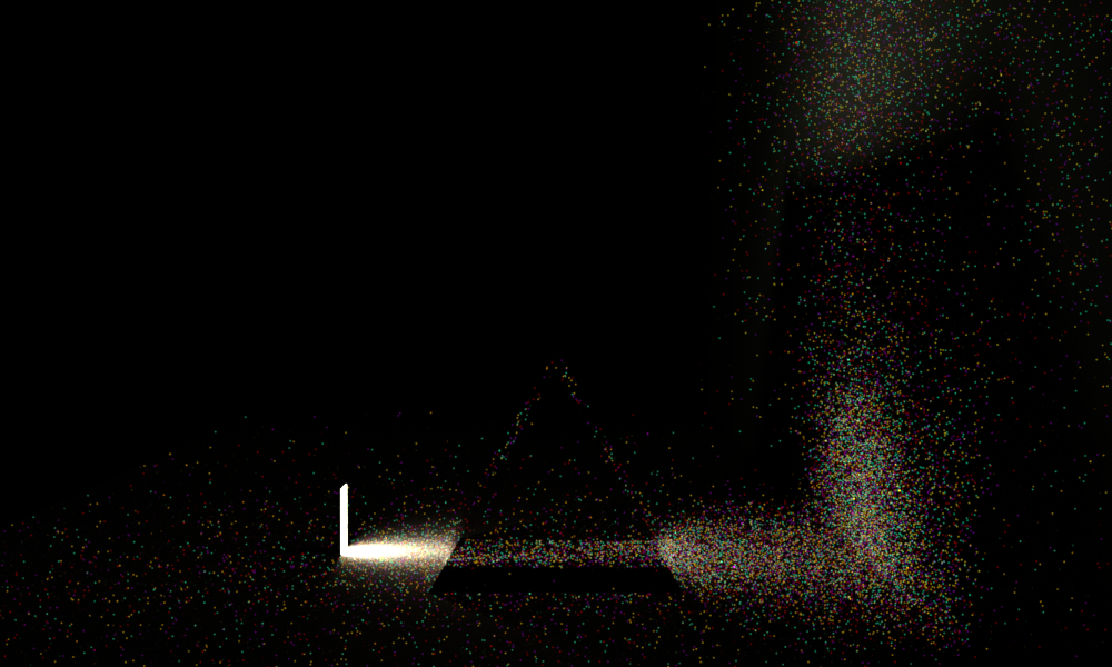
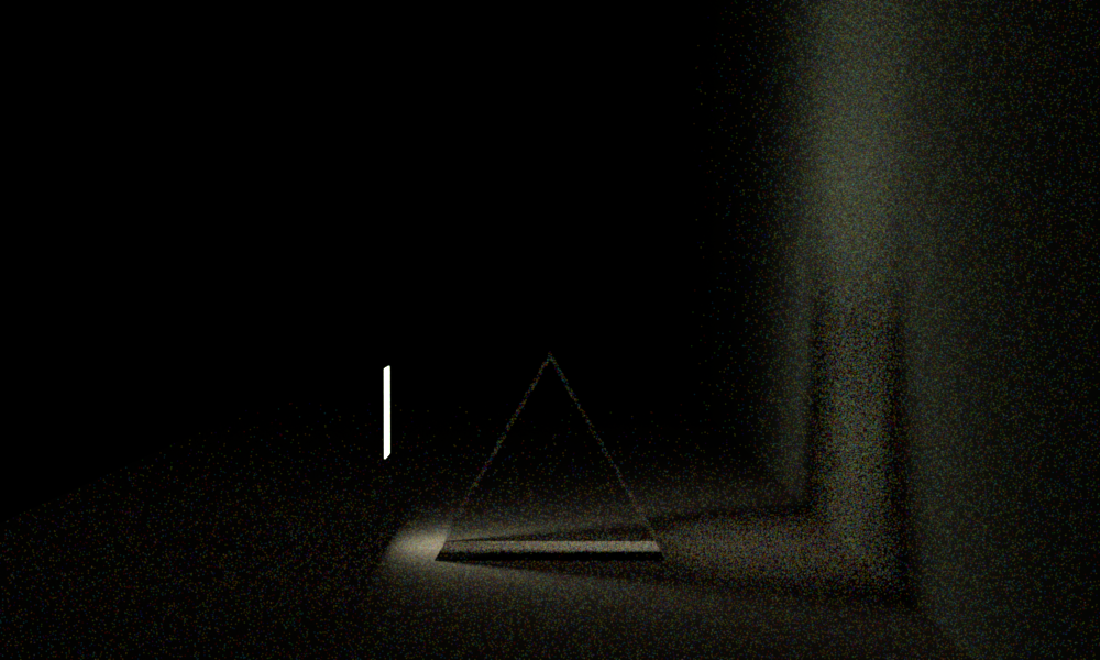
Next we also show a medium with a dielectric ball filled with a medium that has no scattering and no absorption. We show this because it shows how light traverses through the medium (because it's a beautiful image).
Spectral Rendering (15)
Relevant Files
src/spectrum.h, src/spectrum.cpp, src/spectrum_path_mis.cppImplementation
To implement spectral rendering, we extend nori by a Spectrum datatype. This datatype defines all required operators, such as addition, multiplication etc and stores an array that represents the sampled spectrum. In the implementation of the spectrum datatype we very closely follow the implementation in PBRT . We also provide functionality to convert between our Color3f datatype and the spectrum datatype, such that we can re-use all emitters implemented so far. Additionally, our spectrum class provides functionality to sample a random wavelength within the visible spectrum. We will later use this function in the spectral path tracer to have each ray carry a random wavelength.
To be able to use the spectrum datatype, we implement a spectral path tracer that operates on spectra instead of colors. The main idea follows the implementation of path_mis that was implemented as part of the assignments. In our first approach, we sampled a single wavelength per ray. This however creates a lot of colored noise. We therefore sample multiple wavelengths per ray, and then average the resulting spectra together. To reduce computation time, we only sample four random wavelengths along the whole spectrum for this project. However, this could easily be extended to support more wavelengths.
For each ray, we convert the wavelength to its corresponding color using an adaptation of this function, and create a spectrum that corresponds to this color. Since we have all the operations that Color3f has implemented for Spectrum, we can then simply perform path tracing with multiple importance sampling, where every time we would perform an operation on a Color3f, we now perform the corresponding operation on a Spectrum. Whenever we hit an emitter, we multiply the spectrum resulting of the emitter evaluation color with the spectrum corresponding to our current wavelength in order to account for emitter intensity.
To support dielectrics, we also implement a wavelength dependent dielectric bsdf. To do this, we extend the existing bsdf definition by a wavelength dependent sample function. This sample function will just call the wavelength independent sample function by default, such that we can also reuse existing bsdfs in the spectral path tracer. Bsdfs that make use of the wavelength can then simply overwrite this wavelength dependent sample function.
We implement the dielectric, but it could also be extended to wavelength dependent reflectances on diffuse surfaces. To do so, we have implemented a method that returns the wavelength dependent IOR for selected materials. To compute that, we use the functions provided here. So far, we only support a few types of material, but that can easily be extended by adding the corresponding function to compute the IOR.
Validation
Since spectral rendering is not supported by any of the renderers we found, we will just show some images resulting from rendering using the spectral renderer. Below we show a rendering rendered with the spectral path tracer and compare it to one that was rendered using path mis. It has to be noted that the spectral path tracer took about 10 hours to render, while the non-spectral path tracer was finished within a few minutes.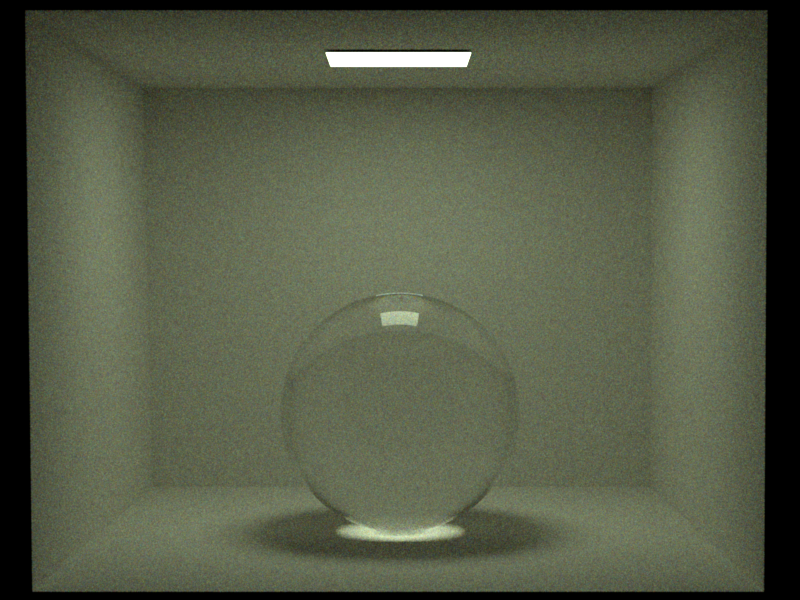
To make dispersion more visible, we provide two more renderings below. We once show the image using a higher radiance, but shorter rendering time, and once using a smaller radiance, but longer rendering time (about 10 hours). Note that this samples 4 fixed wavelengths per ray instead of random. Due to the long computation times, there was however no time to re-render. The results using random wavelengths could however be expected quite similar.
Final Image
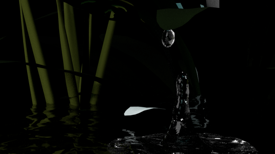
Our scene was inspired by nature. We wanted to play with different textures, surfaces, lighting. We chose a drop of water falling right off a leaf in the forest at night. A scene we would never be able to observe, which is why we chose to render it. We combined meshes of plants, a surface we use as water, and a mesh of a waterdrop with a few emitters. The main challenge was to get just enough light to observe the scene, but not too much as to destroy the atmosphere of the calm night.
Sources:
For our final image, we had to render water. To do this, we used a mesh we got online and added a dielectric bsdf to it. Additionally we use a waterdrop mesh, that also has a dielectric. To model the plants we partly rely on textures that were provided with the plant, but some of them are rendered using different disney bsdf parameters. To get a more realistic overall appearance, we render a background using our environment map feature.
The plants are downloaded from here, converted from 3ds to obj using this converter. The ocean mesh and the mesh for the waterdrop are from Turbosquid. The scene files and .obj fies can be found in the /final_scene folder.